Gaussian Mixture Models with TensorFlow Probability
Content
- Statistics
- Gaussian
- Multivariate Gaussian
- Gaussian Mixture Model
- Multivariate Gaussian Mixture Model
- Conditional Gaussian Mixture Model
In probability theory, a normal (or Gaussian or Gauss or Laplace–Gauss) distribution is a type of continuous probability distribution for a real-valued random variable. — Wikipedia
Dependencies
The required dependencies are Python 3.8, Numpy, Pandas, Matplotlib, TensorFlow, and Tensorflow-Probability.
import numpy as np
import pandas as pd
import matplotlib.pyplot as plt
from mpl_toolkits import mplot3d
import scipy
import tensorflow as tf
import tensorflow_probability as tfp
tfd = tfp.distributions
Statistics
The statistics required are: mean, covariance, diagonal, and standard deviation. We first generate X, a 2D array, then use the Numpy methods to compare statistics against the parameters used.
np.random.seed(0)  # random seed
mu = [0,1]
cov = [[2,0],
       [0,2]]
X = np.random.multivariate_normal(mu, cov, size=100)
X_mean = np.mean(X, axis=0)
X_cov = np.cov(X, rowvar=0)
X_diag = np.diag(X_cov)
X_stddev = np.sqrt(X_diag)
# X_mean
[-9.57681805e-04  1.14277867e+00]
# X_cov
[[ 1.05494742 -0.02517201]
 [-0.02517201  1.04230397]]
# X_diag
[1.05494742 1.04230397]
# X_stddev
[1.02710633 1.02093289]
Notice that the values of mean and covariance computed from X are comparable to the parameters specified to generate X. np.cov uses the parameter rowvar=0 to convert rows of samples into rows of variables to compute the covariance matrix. np.diag obtains the diagonal, which is the variances from a covariance matrix. np.sqrt will obtain the standard deviations of the diagonal.
Gaussian
The Gaussian distribution is defined by its probability density function:
\[p(x) = \frac{1}{\sigma\sqrt{2\pi}} e^{-\frac{1}{2}(\frac{x-\mu}{\sigma})^2}\]
Multivariate Gaussian
The multivariate Gaussian can be modelled using tfd.MultivariateNormalFullCovariance, parameterised by loc and covariance_matrix.
mvn = tfd.MultivariateNormalFullCovariance(
 loc=X_mean,
 covariance_matrix=X_cov)
mvn_mean = mvn.mean().numpy()
mvn_cov = mvn.covariance().numpy()
mvn_stddev = mvn.stddev().numpy()
# mvn_mean
[-0.00135437  1.20191953]
# mvn_cov
[[ 2.10989483 -0.05034403]
 [-0.05034403  2.08460795]]
# mvn_stddev
[1.4525477  1.44381714]
However, tfd.MultivariateNormalFullCovariance will be deprecated and MultivariateNormalTril(loc=loc, scale_tril=tf.linalg.cholesky(covariance_matrix)) should be used instead. Cholesky decomposition of a positive definite matrix (e.g. covariance matrix) can be interpreted as the “square root” of a positive definite matrix [1][2].
# Due to deprecated MultivariateNormalFullCovariance
mvn = tfd.MultivariateNormalTriL(
 loc=X_mean,
 scale_tril=tf.linalg.cholesky(X_cov))
mvn_mean = mvn.mean().numpy()
mvn_cov = mvn.covariance().numpy()
mvn_stddev = mvn.stddev().numpy()
# mvn_mean
[-0.00135437  1.20191953]
# mvn_cov
[[ 2.10989483 -0.05034403]
 [-0.05034403  2.08460795]]
# mvn_stddev
[1.4525477  1.44381714]
Instead of specifying the covariance matrix, the standard deviation can be specified for tfd.MultivariateNormalDiag.
mvn = tfd.MultivariateNormalDiag(
 loc=X_mean,
 scale_diag=X_stddev)
mvn_mean = mvn.mean().numpy()
mvn_cov = mvn.covariance().numpy()
mvn_stddev = mvn.stddev().numpy()
# mvn_mean
[-0.00135437  1.20191953]
# mvn_cov
[[2.10989483 0.        ]
 [0.         2.08460795]]
# mvn_stddev
[1.4525477  1.44381714]
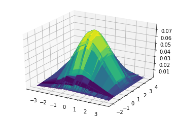
To visualise the probability density function for the multivariate Gaussian, plt.contour can be used.
x1, x2 = np.meshgrid(X[:,0], X[:,1])
data = np.stack((x1.flatten(), x2.flatten()), axis=1)
prob = mvn.prob(data).numpy()
ax = plt.axes(projection='3d')
ax.plot_surface(x1, x2, prob.reshape(x1.shape), cmap='viridis')
plt.show()
Gaussian Mixture Model
The Gaussian mixture model (GMM) is a mixture of Gaussians, each parameterised by by $\mu_k$ and $\sigma_k$, and linearly combined with each component weight, $\theta_k$, that sum to 1. The GMM can be defined by its probability density function:
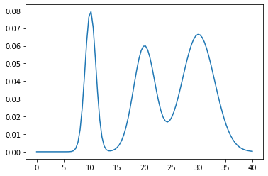
\[p(x) = \sum_{k=1}^K \theta_k\cdot N(x\vert\mu,\sigma)\]Take a mixture of Gaussians parameterised by pi=[0.2,0.3,0.5], mu=[10,20,30], and sigma=[1,2,3]. A categorical distribution tfd.Categorical(probs=pi) is a discrete probability distribution that models a random variable that takes 1 of K possible categories.
pi = np.array([0.2, 0.3, 0.5], dtype=np.float32)
mu = np.array([10, 20, 30], dtype=np.float32)
sigma = np.array([1, 2, 3], dtype=np.float32)
gmm = tfd.Mixture(
    cat=tfd.Categorical(probs=pi),
    components=[tfd.Normal(loc=m, scale=s) for m, s in zip(mu, sigma)]
)
x = np.linspace(0, 40, 100)
plt.plot(x, gmm.prob(x).numpy());
print(gmm.mean().numpy())  # 23.0
tfd.MixtureSameFamily allows definition of mixture models of the same family distribution without a for-loop.
gmm = tfd.MixtureSameFamily(
    mixture_distribution=tfd.Categorical(probs=pi),
    components_distribution=tfd.Normal(loc=mu, scale=sigma)
)
gmm.mean().numpy()  # 23.0
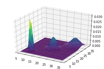
Multivariate Gaussian Mixture Model
Multivariate Gaussian mixture models can be implemented using TensorFlow-Probability by combining tfd.MixtureSameFamily with tfd.MultivariateNormalDiag.
pi = np.array([0.2, 0.3, 0.5], dtype=np.float32)
mu = np.array([[10, 10],
               [20, 20],
               [30, 30]], dtype=np.float32)
sigma = np.array([[1, 1],
                  [2, 2],
                  [3, 3]], dtype=np.float32)
mvgmm = tfd.MixtureSameFamily(
    mixture_distribution=tfd.Categorical(probs=pi),
    components_distribution=tfd.MultivariateNormalDiag(
        loc=mu,
        scale_diag=sigma)
)
x = np.linspace(5, 35, 100)
y = np.linspace(5, 35, 100)
x, y = np.meshgrid(x, y)
data = np.stack((x.flatten(), y.flatten()), axis=1)
prob = mvgmm.prob(data).numpy()
ax = plt.axes(projection='3d')
plt.contour(x, y, prob.reshape((100, 100)));
ax.plot_surface(x, y, prob.reshape((100,100)), cmap='viridis');
Conditional Multivariate Gaussian
Unfortunately, TensorFlow-Probability does not provide support for obtaining the conditional and marginal distributions given the selected features of X. We can implement this ourselves by extending tfd.MultivariateNormalTriL.
def invert_indices(n_features, indices):
    inv = np.ones(n_features, dtype=np.bool)
    inv[indices] = False
    inv, = np.where(inv)
    return inv
class ConditionalMultivariateNormal(tfd.MultivariateNormalTriL):
    def parameters(self):
        covariances = self.covariance()
        means = self.loc
        return means, covariances

    def condition(self, i2, x):
        mu, cov = self.loc, self.covariance()
        i1 = invert_indices(mu.shape[0], indices)

        cov_12 = tf.gather(tf.gather(cov, i1, axis=0), i2, axis=1)
        cov_11 = tf.gather(tf.gather(cov, i1, axis=0), i1, axis=1)
        cov_22 = tf.gather(tf.gather(cov, i2, axis=0), i2, axis=1)

        prec_22 = tf.linalg.pinv(cov_22)
        regression_coeffs = tf.tensordot(cov_12, prec_22, axes=1)

        mean = tf.gather(mu, i1, axis=0)
        diff = tf.transpose(x - tf.gather(mu, i2, axis=0))
        mean += tf.transpose(tf.tensordot(regression_coeffs, diff, axes=1))

        covariance = cov_11 - tf.tensordot(regression_coeffs, tf.transpose(cov_12), axes=0)
        return ConditionalMultivariateNormal(loc=mean, scale_tril=tf.linalg.cholesky(covariance))
    def marginalize(self, indices):
        mu, cov = self.loc, self.covariance()
        return ConditionalMultivariateNormal(loc=mu.numpy()[indices], scale_tril=tf.linalg.cholesky(cov.numpy()[np.ix_(indices, indices)]))
# Conditional Distribution P(X1|X0)
mvn = ConditionalMultivariateNormal(
    loc=X_mean,
    scale_tril=tf.linalg.cholesky(X_cov))
x = np.array([2])
indices = np.array([1])
conditional_mvn = mvn.condition(indices, x)
marginal_mvn = mvn.marginalize(indices)
print(conditional_mvn.sample().numpy())
print(marginal_mvn.sample().numpy())
# Conditional MVN sample
[[[[1.60346902]]]
 [[[0.70901248]]]
 [[[0.68173244]]]]
# Marginal MVN sample
[[-0.22300554]
 [ 2.69431439]
 [-0.52467359]]